A useful mental model for thinking about large language models is that they are very large lookup tables. During training, they compress an enormous amount of information about language and the world into billions of floating-point weights. During inference, they recall and recombine relevant parts of that compressed knowledge to generate a response.
The uncomfortable implication of this model is that making the lookup table bigger – training more parameters – should produce better recall. And empirically, within the regime described by scaling laws, it does. But a larger table is also more expensive to consult. If every token you generate requires a forward pass through 70 billion parameters, the compute cost is substantial and the latency is real.
Mixture of Experts is the architectural answer to this tension. It asks: what if you had a very large table, but only looked up a small portion of it for each query?
The Basic Architecture
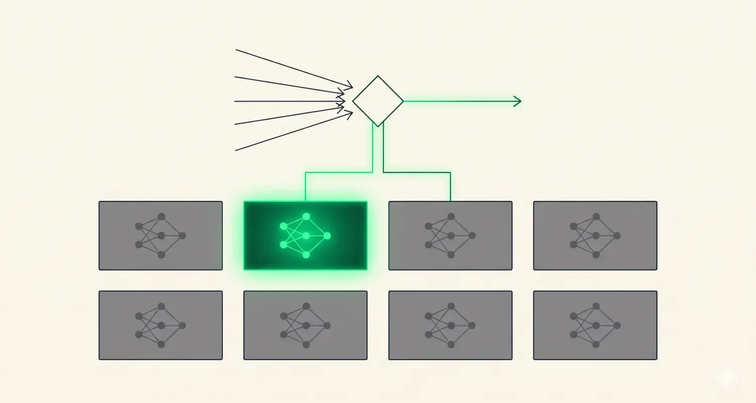
A Mixture of Experts model replaces some or all of the dense feed-forward layers in a transformer with a MoE layer. Each MoE layer contains multiple parallel sub-networks called experts – typically between 8 and 64 in current models. It also contains a small learned network called the router or gating network.
For each input token, the router examines the token’s representation and selects a small number of experts – usually 2 out of the total pool – to process it. Only those selected experts perform computation. The outputs of the selected experts are weighted by the router’s confidence scores and combined.
The key numbers: a Mixtral 8x7B model has 8 experts per layer, each of which is a 7B-parameter-scale feed-forward network. But only 2 experts are activated per token. The total parameter count is around 47 billion – but the active parameter count during any forward pass is closer to 13 billion.
You get 47 billion parameters worth of capacity. You pay 13 billion parameters worth of compute. This is the central trade-off that makes MoE attractive.
The Router and the Load Balancing Problem
The router is a learned linear layer with a softmax output. Given the hidden representation of a token, it produces a probability distribution over all available experts and selects the top-k. The selected experts process the token; the others do nothing.
In theory, the router learns to specialize experts – sending mathematical tokens to experts that have become good at mathematics, code tokens to code-oriented experts, and so on. There is some evidence that this specialization does occur in practice, though it is less cleanly delineated than the intuition suggests.
In practice, the router creates a significant training challenge: it wants to collapse. The router quickly learns that some experts produce slightly better outputs than others and begins routing all tokens to those experts, leaving the rest idle. You end up paying for the capacity of 8 experts but training only 2 of them.
The standard solution is an auxiliary load-balancing loss that penalizes uneven expert utilization. This loss pushes the router toward distributing tokens more evenly across experts. It introduces a tension with the main training objective – the router wants to send tokens to the best experts, but the auxiliary loss pushes it toward uniform distribution – and the balance between these objectives is a hyperparameter that requires care.
More recent work has explored alternative routing strategies. Expert Choice routing inverts the relationship: instead of tokens choosing experts, each expert chooses which tokens to process, selecting its top-k from the batch. This guarantees perfect load balancing by construction, but introduces the complication that different tokens may be processed by different numbers of experts, making batching less straightforward.
Communication Overhead in Distributed Training
One of the less-discussed costs of MoE is that it is genuinely harder to train efficiently at scale.
Dense models distribute parameters across GPUs in relatively straightforward ways. With MoE, you need to route tokens to the GPU that holds the relevant expert – which may not be the GPU that originally held the token. This requires all-to-all communication between GPUs, where every device sends data to every other device.
All-to-all communication does not scale as cleanly as point-to-point communication. As you add more GPUs, the communication overhead grows, and network bandwidth becomes a bottleneck that can partially offset the compute savings. The practical benefit of MoE is therefore sensitive to the ratio of compute speed to network bandwidth in your hardware configuration.
This is one reason why MoE has been more practically successful in research settings with high-bandwidth interconnects – NVLink, InfiniBand – than in more loosely coupled distributed systems.
What the Evidence Shows
The evidence for MoE is strong enough that it has been adopted by several of the most capable publicly available models.
Mixtral 8x7B, released by Mistral AI in 2023, demonstrated that a sparse MoE model with 13 billion active parameters could match or exceed the performance of Llama 2 70B – a dense model requiring roughly 5× the active compute – on most standard benchmarks. The inference cost advantage is significant in deployment.
Google’s Gemini 1.5 is reported to use a MoE architecture, though the specifics have not been fully disclosed. GPT-4 is widely believed to be a MoE model, again without official confirmation. The pattern suggests that at the frontier of model capability, sparse architectures are becoming standard practice rather than an experimental alternative.
The Capacity vs. Compute Decoupling
The deeper significance of MoE is what it implies about the relationship between model capacity and inference cost – a relationship that dense models force to be fixed.
In a dense model, if you want more capacity, you add more parameters, and every forward pass becomes proportionally more expensive. The scaling law tradeoff is locked in at training time.
MoE decouples these. You can scale capacity by adding more experts without increasing the per-token compute, up to the limits imposed by routing overhead and memory. Conversely, if you have a fixed inference budget, you can use a MoE architecture to afford a much richer parameter space than a dense model would allow.
This is not unlimited. You cannot add experts indefinitely without eventually hitting diminishing returns, and the memory required to store all experts must fit somewhere – which at 47 billion parameters means at minimum several A100s even for inference. But the principle is sound, and the practical results show it works.
The open question is how far the scaling can go. Current models use tens to low-hundreds of experts per layer. Whether architectures with thousands of fine-grained experts, or dynamic expert creation, or hierarchical routing, can push the frontier further is an active area of research with no settled answer.
What is settled is that the era of every parameter being active on every forward pass is ending. The next generation of large models is likely to be even more sparsely activated – not because sparsity is inherently elegant, but because the compute economics strongly favor it.