The Vanishing Gradient Problem – Why Deep Networks Forget Where They Came From

There is a paradox buried in the design of deep neural networks. The deeper you make a network, the more expressive it should become – more layers means more capacity to represent complex functions. And yet, for most of the 2000s, training networks deeper than five or six layers reliably produced models that performed worse than their shallower counterparts.

The culprit had a name by the early 1990s: the vanishing gradient problem. Understanding it is not just a history lesson. It explains why almost every architectural decision in modern deep learning – residual connections, normalization layers, careful initialization schemes — exists.

Backpropagation and the Chain Rule

To understand why gradients vanish, you first need to understand how they move through a network.

Training a neural network means adjusting its weights to reduce some loss function. We do this by computing the gradient of the loss with respect to every weight in the network – a number that tells us how much a small change in that weight would increase or decrease the loss. Backpropagation computes these gradients efficiently using the chain rule of calculus.

The chain rule says: if you want to know how the loss changes with respect to a weight in layer one, you multiply together the local gradients at every layer between layer one and the output. In a network with ten layers, the gradient at layer one is a product of ten terms.

This is where the problem lives.

Why the Product Collapses

In the early days of neural networks, the activation function of choice was the sigmoid: a smooth S-shaped curve that squashes any input into the range (0, 1). It was biologically motivated, differentiable everywhere, and seemed well-behaved.

The problem is what happens to its derivative. The sigmoid’s gradient is maximized at zero input, where it reaches exactly 0.25. Everywhere else it is smaller – and for large positive or negative inputs, it approaches zero rapidly. This is called saturation: neurons with large activations have near-zero gradients.

Now consider backpropagation through ten such layers. At each layer, the gradient is multiplied by the local sigmoid derivative – a number almost always less than 0.25. After ten multiplications, you have at most 0.25¹⁰ ≈ 0.000001. In practice it is often far smaller, because weights are involved in the multiplication too.

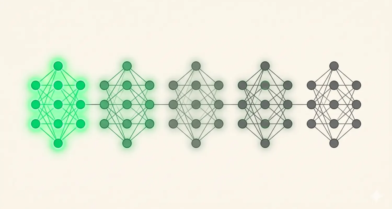
By the time the gradient reaches the earliest layers, it is so small it is numerically indistinguishable from zero. Those layers receive no meaningful learning signal. They do not update. The network effectively learns only in its last few layers, no matter how deep you make it.

The opposite problem – exploding gradients – occurs when those multiplied terms are greater than one, sending gradients to infinity. This was particularly acute in recurrent networks processing long sequences, where the same weight matrix is multiplied by itself hundreds of times.

What Researchers Tried

The first generation of solutions attacked the problem at the activation function. In 2010, Xavier Glorot and Yoshua Bengio published a careful study of how activation functions and initialization interact with gradient flow. Shortly after, the ReLU – Rectified Linear Unit – began its rise to dominance.

ReLU is almost embarrassingly simple: output the input if it is positive, output zero otherwise. Its derivative is either 1 (for positive inputs) or 0. That constant derivative of 1 for active neurons means gradients pass through ReLU layers without being attenuated. A chain of ten ReLU layers multiplies gradients by ten ones rather than ten quarter-fractions.

This was a significant improvement. Networks with ReLU activations trained faster and reached better performance than their sigmoid counterparts. But it did not eliminate the problem – it just pushed the workable depth from roughly five layers to roughly twenty before training became unreliable again.

The Residual Connection

The real breakthrough came in 2015, from a Microsoft Research team led by Kaiming He. Their paper introduced the residual network – ResNet – and demonstrated something that seemed impossible at the time: a 152-layer network that was also the best-performing model on ImageNet that year.

The key idea is the skip connection, or residual connection. Instead of asking each layer to learn a complete transformation of its input, you ask it to learn only the residual – the difference between the input and the desired output. The input is then added back to the layer’s output before passing it on.

Mathematically, where a standard layer computes H(x), a residual block computes H(x) = F(x) + x, where F(x) is what the layer actually learns. If the optimal transformation is close to the identity – the layer should mostly leave its input alone – then F(x) should be close to zero, which is easy to learn. But more importantly, the addition creates a direct path for gradients to flow backward through the network without passing through any nonlinearity.

During backpropagation, the gradient of a residual block is the gradient from the next layer plus the gradient flowing through the skip connection directly. Even if the learned path has near-zero gradient, the skip connection carries a full-strength gradient straight back to earlier layers. No matter how deep the network, the earliest layers always receive at least some gradient signal.

Normalization Layers

Running alongside residual connections, batch normalization – introduced by Ioffe and Szegedy in 2015 – solved a related problem. During training, the distribution of activations at any layer shifts constantly as the weights of previous layers change. This internal covariate shift means each layer is always trying to hit a moving target.

Batch normalization normalizes the activations at each layer to have zero mean and unit variance, then applies learned scale and shift parameters. This keeps activations in the regime where gradients are well-behaved, substantially reduces the sensitivity to initialization, and allows much higher learning rates.

Layer normalization – a variant that normalizes across features rather than batch samples – later became standard in transformers, where variable sequence lengths make batch normalization awkward.

Where We Are Now

Modern deep learning operates under something like a truce with the vanishing gradient problem. ResNets make it tractable for convolutional networks up to hundreds of layers. Transformers use a combination of layer normalization, residual connections, and attention mechanisms that give gradients many direct paths back to early layers. Careful initialization schemes – Xavier initialization, He initialization – ensure that gradients start in a reasonable range before any learning begins.

The problem has not been solved so much as systematically routed around. Every technique in that list is a structural guarantee that gradients stay alive long enough to do useful work.

Understanding this history matters because these are not arbitrary design choices. They are load-bearing walls. When you encounter a residual connection in a modern architecture diagram and wonder why it is there, the answer is: because without it, the gradient would have vanished long before it reached layer one.